QQ-plot
For a single variable
In order to check the normality assumption of a variable (normality means that the data follow a normal distribution, also known as a Gaussian distribution), we usually use histograms and/or QQ-plots.1 See an article discussing about the normal distribution and how to evaluate the normality assumption in R if you need a refresh on that subject. Histograms have been presented earlier, so here is how to draw a QQ-plot:
# Draw points on the qq-plot:
qqnorm(dat$Sepal.Length)
# Draw the reference line:
qqline(dat$Sepal.Length)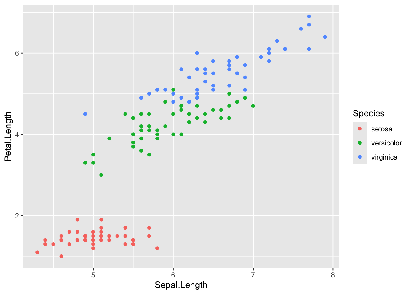
Or a QQ-plot with confidence bands with the qqPlot() function from the {car} package:
library(car) # package must be installed first
qqPlot(dat$Sepal.Length)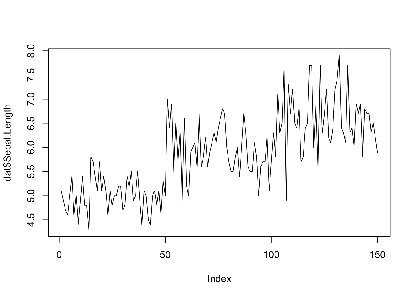
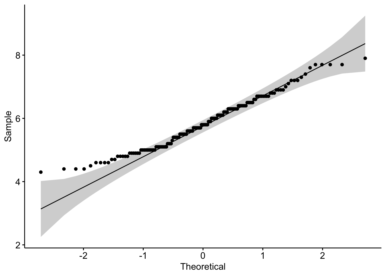
## [1] 132 118If points are close to the reference line (sometimes referred as Henry’s line) and within the confidence bands, the normality assumption can be considered as met. The bigger the deviation between the points and the reference line and the more they lie outside the confidence bands, the less likely that the normality condition is met. The variable Sepal.Length does not seem to follow a normal distribution because several points lie outside the confidence bands. When facing a non-normal distribution, the first step is usually to apply the logarithm transformation on the data and recheck to see whether the log-transformed data are normally distributed. Applying the logarithm transformation can be done with the log() function.
In {ggpubr}:
library(ggpubr)
ggqqplot(dat$Sepal.Length)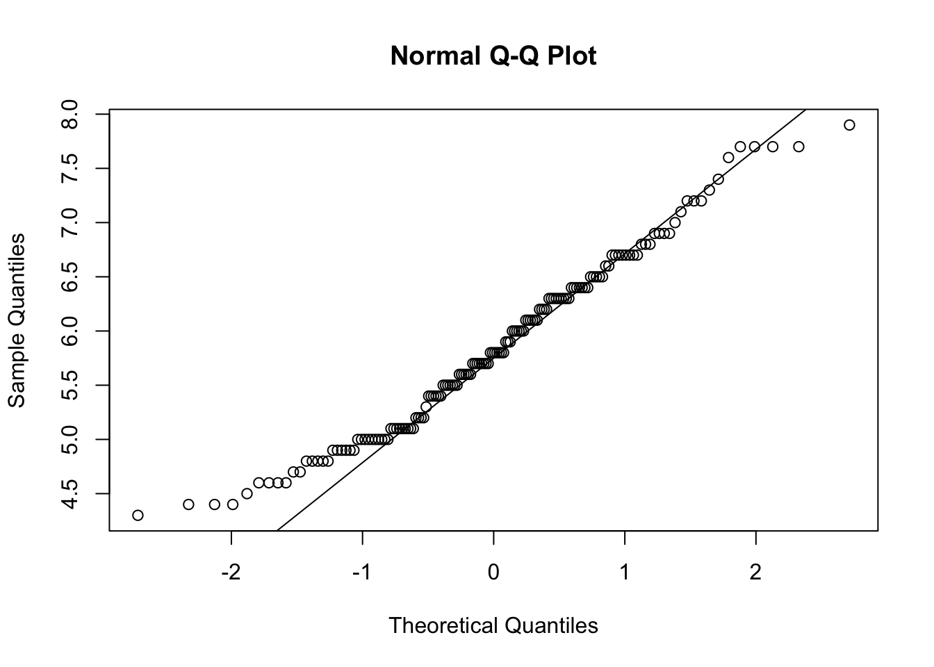
By groups
For some statistical tests, the normality assumption is required in all groups. One solution is to draw a QQ-plot for each group by manually splitting the dataset into different groups and then draw a QQ-plot for each subset of the data (with the methods shown above). Another (easier) solution is to draw a QQ-plot for each group automatically with the argument groups = in the function qqPlot() from the {car} package:
qqPlot(dat$Sepal.Length, groups = dat$size)
In {ggplot2}:
qplot(
  sample = Sepal.Length, data = dat,
  col = size, shape = size
)
It is also possible to differentiate groups by only shape or color. For this, remove one of the argument col or shape in the qplot() function above.
Density plot
Density plot is a smoothed version of the histogram and is used in the same concept, that is, to represent the distribution of a numeric variable. The functions plot() and density() are used together to draw a density plot:
plot(density(dat$Sepal.Length))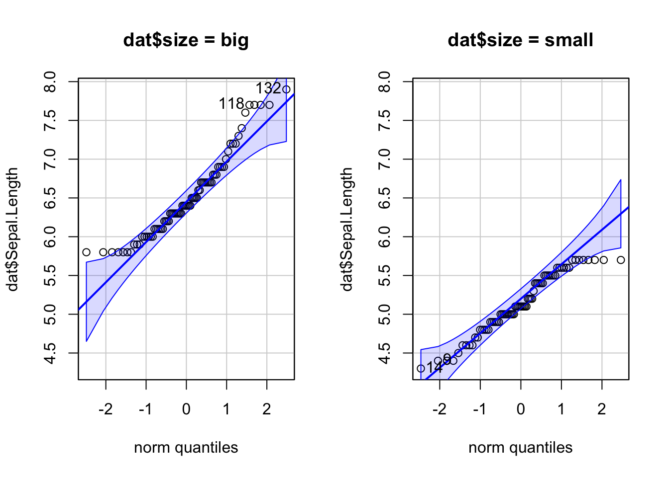
In {ggplot2}:
ggplot(dat) +
  aes(x = Sepal.Length) +
  geom_density()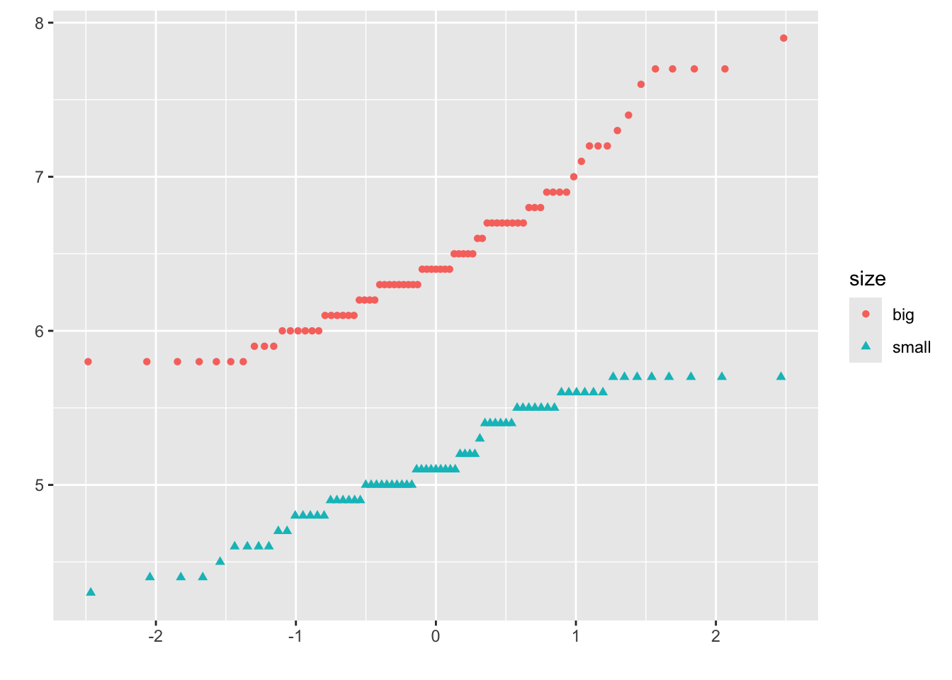
Advanced descriptive statistics
We covered the main functions to compute the most common and basic descriptive statistics. There are, however, many more functions and packages to perform more advanced descriptive statistics in R. In this section, I present some of them with applications to our dataset.
{summarytools} package
One package for descriptive statistics I often use for my projects in R is the {summarytools} package. The package is centered around 4 functions:
freq()for frequencies tablesctable()for cross-tabulationsdescr()for descriptive statisticsdfSummary()for dataframe summaries
A combination of these 4 functions is usually more than enough for most descriptive analyses. Moreover, the package has been built with R Markdown in mind, meaning that outputs render well in HTML reports. And for non-English speakers, built-in translations exist for French, Portuguese, Spanish, Russian and Turkish.
I illustrate each of the 4 functions in the following sections. Outputs that follow display much better in R Markdown reports, but in this article I limit myself to the raw outputs as the goal is to show how the functions work, not how to make them render well. See the setup settings in the vignette of the package if you want to print the outputs in a nice way in R Markdown.2
Frequency tables with freq()
The freq() function produces frequency tables with frequencies, proportions, as well as missing data information.
library(summarytools)
freq(dat$Species)## Frequencies
## dat$Species
## Type: Factor
##
## Freq % Valid % Valid Cum. % Total % Total Cum.
## ---------------- ------ --------- -------------- --------- --------------
## setosa 50 33.33 33.33 33.33 33.33
## versicolor 50 33.33 66.67 33.33 66.67
## virginica 50 33.33 100.00 33.33 100.00
## <NA> 0 0.00 100.00
## Total 150 100.00 100.00 100.00 100.00If you do not need information about missing values, add the report.nas = FALSE argument:
freq(dat$Species,
  report.nas = FALSE # remove NA information
)## Frequencies
## dat$Species
## Type: Factor
##
## Freq % % Cum.
## ---------------- ------ -------- --------
## setosa 50 33.33 33.33
## versicolor 50 33.33 66.67
## virginica 50 33.33 100.00
## Total 150 100.00 100.00And for a minimalist output with only counts and proportions:
freq(dat$Species,
  report.nas = FALSE, # remove NA information
  totals = FALSE, # remove totals
  cumul = FALSE, # remove cumuls
  headings = FALSE # remove headings
)##
## Freq %
## ---------------- ------ -------
## setosa 50 33.33
## versicolor 50 33.33
## virginica 50 33.33Cross-tabulations with ctable()
The ctable() function produces cross-tabulations (also known as contingency tables) for pairs of categorical variables. Using the two categorical variables in our dataset:
ctable(
  x = dat$Species,
  y = dat$size
)## Cross-Tabulation, Row Proportions
## Species * size
## Data Frame: dat
##
## ------------ ------ ------------ ------------ --------------
## size big small Total
## Species
## setosa 1 ( 2.0%) 49 (98.0%) 50 (100.0%)
## versicolor 29 (58.0%) 21 (42.0%) 50 (100.0%)
## virginica 47 (94.0%) 3 ( 6.0%) 50 (100.0%)
## Total 77 (51.3%) 73 (48.7%) 150 (100.0%)
## ------------ ------ ------------ ------------ --------------Row proportions are shown by default. To display column or total proportions, add the prop = "c" or prop = "t" arguments, respectively:
ctable(
  x = dat$Species,
  y = dat$size,
  prop = "t" # total proportions
)## Cross-Tabulation, Total Proportions
## Species * size
## Data Frame: dat
##
## ------------ ------ ------------ ------------ --------------
## size big small Total
## Species
## setosa 1 ( 0.7%) 49 (32.7%) 50 ( 33.3%)
## versicolor 29 (19.3%) 21 (14.0%) 50 ( 33.3%)
## virginica 47 (31.3%) 3 ( 2.0%) 50 ( 33.3%)
## Total 77 (51.3%) 73 (48.7%) 150 (100.0%)
## ------------ ------ ------------ ------------ --------------To remove proportions altogether, add the argument prop = "n". Furthermore, to display only the bare minimum, add the totals = FALSE and headings = FALSE arguments:
ctable(
  x = dat$Species,
  y = dat$size,
  prop = "n", # remove proportions
  totals = FALSE, # remove totals
  headings = FALSE # remove headings
)##
## ------------ ------ ----- -------
## size big small
## Species
## setosa 1 49
## versicolor 29 21
## virginica 47 3
## ------------ ------ ----- -------This is equivalent than table(dat$Species, dat$size) and xtabs(~ dat$Species + dat$size) performed in the section on contingency tables.
To display results of the Chi-square test of independence, add the chisq = TRUE argument:3
ctable(
  x = dat$Species,
  y = dat$size,
  chisq = TRUE, # display results of Chi-square test of independence
  headings = FALSE # remove headings
)##
## ------------ ------ ------------ ------------ --------------
## size big small Total
## Species
## setosa 1 ( 2.0%) 49 (98.0%) 50 (100.0%)
## versicolor 29 (58.0%) 21 (42.0%) 50 (100.0%)
## virginica 47 (94.0%) 3 ( 6.0%) 50 (100.0%)
## Total 77 (51.3%) 73 (48.7%) 150 (100.0%)
## ------------ ------ ------------ ------------ --------------
##
## ----------------------------
## Chi.squared df p.value
## ------------- ---- ---------
## 86.03 2 0
## ----------------------------The p-value is close to 0 so we reject the null hypothesis of independence between the two variables. In our context, this indicates that species and size are dependent and that there is a significant relationship between the two variables.
It is also possible to create a contingency table for each level of a third categorical variable thanks to the combination of the stby() and ctable() functions. There are only 2 categorical variables in our dataset, so let’s use the tabacco dataset which has 4 categorical variables (i.e., gender, age group, smoker, diseased). For this example, we would like to create a contingency table of the variables smoker and diseased, and this for each gender:
stby(list(
  x = tobacco$smoker, # smoker and diseased
  y = tobacco$diseased
),
INDICES = tobacco$gender, # for each gender
FUN = ctable # ctable for cross-tabulation
)## Cross-Tabulation, Row Proportions
## smoker * diseased
## Data Frame: tobacco
## Group: gender = F
##
## -------- ---------- ------------- ------------- --------------
## diseased Yes No Total
## smoker
## Yes 62 (42.2%) 85 (57.8%) 147 (100.0%)
## No 49 (14.3%) 293 (85.7%) 342 (100.0%)
## Total 111 (22.7%) 378 (77.3%) 489 (100.0%)
## -------- ---------- ------------- ------------- --------------
##
## Group: gender = M
##
## -------- ---------- ------------- ------------- --------------
## diseased Yes No Total
## smoker
## Yes 63 (44.1%) 80 (55.9%) 143 (100.0%)
## No 47 (13.6%) 299 (86.4%) 346 (100.0%)
## Total 110 (22.5%) 379 (77.5%) 489 (100.0%)
## -------- ---------- ------------- ------------- --------------Descriptive statistics with descr()
The descr() function produces descriptive (univariate) statistics with common central tendency statistics and measures of dispersion. (See the difference between a measure of central tendency and dispersion if you need a reminder.)
A major advantage of this function is that it accepts single vectors as well as data frames. If a data frame is provided, all non-numerical columns are ignored so you do not have to remove them yourself before running the function.
The descr() function allows to display:
- only a selection of descriptive statistics of your choice, with the
stats = c("mean", "sd")argument for mean and standard deviation for example - the minimum, first quartile, median, third quartile and maximum with
stats = "fivenum" - the most common descriptive statistics (mean, standard deviation, minimum, median, maximum, number and percentage of valid observations), with
stats = "common":
descr(dat,
  headings = FALSE, # remove headings
  stats = "common" # most common descriptive statistics
)
##
## Petal.Length Petal.Width Sepal.Length Sepal.Width
## --------------- -------------- ------------- -------------- -------------
## Mean 3.76 1.20 5.84 3.06
## Std.Dev 1.77 0.76 0.83 0.44
## Min 1.00 0.10 4.30 2.00
## Median 4.35 1.30 5.80 3.00
## Max 6.90 2.50 7.90 4.40
## N.Valid 150.00 150.00 150.00 150.00
## Pct.Valid 100.00 100.00 100.00 100.00Tip: if you have a large number of variables, add the transpose = TRUE argument for a better display.
In order to compute these descriptive statistics by group (e.g., Species in our dataset), use the descr() function in combination with the stby() function:
stby(
  data = dat,
  INDICES = dat$Species, # by Species
  FUN = descr, # descriptive statistics
  stats = "common" # most common descr. stats
)## Descriptive Statistics
## dat
## Group: Species = setosa
## N: 50
##
## Petal.Length Petal.Width Sepal.Length Sepal.Width
## --------------- -------------- ------------- -------------- -------------
## Mean 1.46 0.25 5.01 3.43
## Std.Dev 0.17 0.11 0.35 0.38
## Min 1.00 0.10 4.30 2.30
## Median 1.50 0.20 5.00 3.40
## Max 1.90 0.60 5.80 4.40
## N.Valid 50.00 50.00 50.00 50.00
## Pct.Valid 100.00 100.00 100.00 100.00
##
## Group: Species = versicolor
## N: 50
##
## Petal.Length Petal.Width Sepal.Length Sepal.Width
## --------------- -------------- ------------- -------------- -------------
## Mean 4.26 1.33 5.94 2.77
## Std.Dev 0.47 0.20 0.52 0.31
## Min 3.00 1.00 4.90 2.00
## Median 4.35 1.30 5.90 2.80
## Max 5.10 1.80 7.00 3.40
## N.Valid 50.00 50.00 50.00 50.00
## Pct.Valid 100.00 100.00 100.00 100.00
##
## Group: Species = virginica
## N: 50
##
## Petal.Length Petal.Width Sepal.Length Sepal.Width
## --------------- -------------- ------------- -------------- -------------
## Mean 5.55 2.03 6.59 2.97
## Std.Dev 0.55 0.27 0.64 0.32
## Min 4.50 1.40 4.90 2.20
## Median 5.55 2.00 6.50 3.00
## Max 6.90 2.50 7.90 3.80
## N.Valid 50.00 50.00 50.00 50.00
## Pct.Valid 100.00 100.00 100.00 100.00Data frame summaries with dfSummary()
The dfSummary() function generates a summary table with statistics, frequencies and graphs for all variables in a dataset. The information shown depends on the type of the variables (character, factor, numeric, date) and also varies according to the number of distinct values.
dfSummary(dat)## Data Frame Summary
## dat
## Dimensions: 150 x 6
## Duplicates: 1
##
## ----------------------------------------------------------------------------------------------------------------------
## No Variable Stats / Values Freqs (% of Valid) Graph Valid Missing
## ---- --------------- ------------------------ -------------------- -------------------------------- -------- ---------
## 1 Sepal.Length Mean (sd) : 5.8 (0.8) 35 distinct values . . : : 150 0
## [numeric] min < med < max: : : : : (100%) (0%)
## 4.3 < 5.8 < 7.9 : : : : :
## IQR (CV) : 1.3 (0.1) : : : : :
## : : : : : : : :
##
## 2 Sepal.Width Mean (sd) : 3.1 (0.4) 23 distinct values : 150 0
## [numeric] min < med < max: : (100%) (0%)
## 2 < 3 < 4.4 . :
## IQR (CV) : 0.5 (0.1) : : : :
## . . : : : : : :
##
## 3 Petal.Length Mean (sd) : 3.8 (1.8) 43 distinct values : 150 0
## [numeric] min < med < max: : . : (100%) (0%)
## 1 < 4.3 < 6.9 : : : .
## IQR (CV) : 3.5 (0.5) : : : : : .
## : : . : : : : : .
##
## 4 Petal.Width Mean (sd) : 1.2 (0.8) 22 distinct values : 150 0
## [numeric] min < med < max: : (100%) (0%)
## 0.1 < 1.3 < 2.5 : . . :
## IQR (CV) : 1.5 (0.6) : : : : .
## : : : : : . : : :
##
## 5 Species 1. setosa 50 (33.3%) IIIIII 150 0
## [factor] 2. versicolor 50 (33.3%) IIIIII (100%) (0%)
## 3. virginica 50 (33.3%) IIIIII
##
## 6 size 1. big 77 (51.3%) IIIIIIIIII 150 0
## [character] 2. small 73 (48.7%) IIIIIIIII (100%) (0%)
## ----------------------------------------------------------------------------------------------------------------------describeBy() from the {psych} package
The describeBy() function from the {psych} package allows to report several summary statistics (i.e., number of valid cases, mean, standard deviation, median, trimmed mean, mad: median absolute deviation (from the median), minimum, maximum, range, skewness and kurtosis) by a grouping variable.
library(psych)
describeBy(
  dat,
  dat$Species # grouping variable
)
##
## Descriptive statistics by group
## group: setosa
## vars n mean sd median trimmed mad min max range skew kurtosis
## Sepal.Length 1 50 5.01 0.35 5.0 5.00 0.30 4.3 5.8 1.5 0.11 -0.45
## Sepal.Width 2 50 3.43 0.38 3.4 3.42 0.37 2.3 4.4 2.1 0.04 0.60
## Petal.Length 3 50 1.46 0.17 1.5 1.46 0.15 1.0 1.9 0.9 0.10 0.65
## Petal.Width 4 50 0.25 0.11 0.2 0.24 0.00 0.1 0.6 0.5 1.18 1.26
## Species* 5 50 1.00 0.00 1.0 1.00 0.00 1.0 1.0 0.0 NaN NaN
## size* 6 50 NaN NA NA NaN NA Inf -Inf -Inf NA NA
## se
## Sepal.Length 0.05
## Sepal.Width 0.05
## Petal.Length 0.02
## Petal.Width 0.01
## Species* 0.00
## size* NA
## ------------------------------------------------------------
## group: versicolor
## vars n mean sd median trimmed mad min max range skew
## Sepal.Length 1 50 5.94 0.52 5.90 5.94 0.52 4.9 7.0 2.1 0.10
## Sepal.Width 2 50 2.77 0.31 2.80 2.78 0.30 2.0 3.4 1.4 -0.34
## Petal.Length 3 50 4.26 0.47 4.35 4.29 0.52 3.0 5.1 2.1 -0.57
## Petal.Width 4 50 1.33 0.20 1.30 1.32 0.22 1.0 1.8 0.8 -0.03
## Species* 5 50 2.00 0.00 2.00 2.00 0.00 2.0 2.0 0.0 NaN
## size* 6 50 NaN NA NA NaN NA Inf -Inf -Inf NA
## kurtosis se
## Sepal.Length -0.69 0.07
## Sepal.Width -0.55 0.04
## Petal.Length -0.19 0.07
## Petal.Width -0.59 0.03
## Species* NaN 0.00
## size* NA NA
## ------------------------------------------------------------
## group: virginica
## vars n mean sd median trimmed mad min max range skew
## Sepal.Length 1 50 6.59 0.64 6.50 6.57 0.59 4.9 7.9 3.0 0.11
## Sepal.Width 2 50 2.97 0.32 3.00 2.96 0.30 2.2 3.8 1.6 0.34
## Petal.Length 3 50 5.55 0.55 5.55 5.51 0.67 4.5 6.9 2.4 0.52
## Petal.Width 4 50 2.03 0.27 2.00 2.03 0.30 1.4 2.5 1.1 -0.12
## Species* 5 50 3.00 0.00 3.00 3.00 0.00 3.0 3.0 0.0 NaN
## size* 6 50 NaN NA NA NaN NA Inf -Inf -Inf NA
## kurtosis se
## Sepal.Length -0.20 0.09
## Sepal.Width 0.38 0.05
## Petal.Length -0.37 0.08
## Petal.Width -0.75 0.04
## Species* NaN 0.00
## size* NA NAaggregate() function
The aggregate() function allows to split the data into subsets and then to compute summary statistics for each. For instance, if we want to compute the mean for the variables Sepal.Length and Sepal.Width by Species and Size:
aggregate(cbind(Sepal.Length, Sepal.Width) ~ Species + size,
  data = dat,
  mean
)
## Species size Sepal.Length Sepal.Width
## 1 setosa big 5.800000 4.000000
## 2 versicolor big 6.282759 2.868966
## 3 virginica big 6.663830 2.997872
## 4 setosa small 4.989796 3.416327
## 5 versicolor small 5.457143 2.633333
## 6 virginica small 5.400000 2.600000
0 comments:
Post a Comment